Module 1—Motion
 Reflect and Connect
The following data table shows the altitude of the shuttle during launch. Use this data and your graphing skills to illustrate the vertical velocity and acceleration of the vehicle in the first minute and one-half of the launch. In other words, draw a position-time graph. From that, draw the velocity-time graph. Use the velocity-time graph to draw the acceleration-time graph.
Time (s) |
Altitude (m) |
0 |
0 |
10 |
560 |
20 |
2240 |
30 |
5040 |
40 |
8960 |
50 |
14 000 |
60 |
20 160 |
70 |
27 440 |
80 |
35 840 |
90 |
45 360 |
Can you connect this with how it must have felt to have been in the shuttle at these different times? What would have been the most exciting point during liftoff? Why?
 Discuss
Prepare to share and compare your shuttle altitude and experience graphs with others. Use this question as a starting point for discussion: Where would the best thrill point or extreme experience be during the liftoff?
 Going Beyond

© Image courtesy of Shutterstock.com
You are programming a control computer for a subway train with the following parameters.
- The train can accelerate from rest (v = 0.0 m/s) at 2.00 m/s2.
- The maximum speed of the train is 30.0 m/s.
- The train can brake at 3.00 m/s2.
-
The total distance that the subway car travels between stops is 1.0 km.
 Try This
TR 4. Use the following questions and the graphing capabilities of the simulation to help create motion scripts that could accomplish this.
-
How much time is required to accelerate from rest at 2.00 m/s2 in order to achieve the maximum speed?
-
How far does the subway train travel while accelerating up to the maximum speed?
-
How long will it take the train to stop if it starts at the maximum speed and accelerates at 3.00 m/s2?
-
How far does the subway train travel while stopping?
-
Given the starting and stopping distances, how far and how long does the train travel at the maximum speed? (Hint: Use the answers for TR 4.b. and TR 4.d. to help you answer the question.)
-
How much time will it take for the subway train to travel between stops?
-
What is the average speed of the train as it travels between stops?
-
Give the three motion scripts that will be used to control the train.
time: ______ s, initial velocity: ______ m/s, acceleration: ______ m/s2
time: ______ s, initial velocity: ______ m/s, acceleration: ______ m/s2
time: ______ s, initial velocity: ______ m/s, acceleration: ______ m/s2
-
Complete all three graphs that illustrate the train's motion.
Position-Time
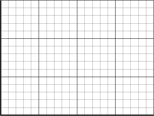
Velocity-Time

Acceleration-Time

 Reflect on the Big Picture
In this lesson you saw again how graphs assist you as you try to describe how objects are moving. You used graphs and some of their features to solve problems. Did you see how the concepts here built on the ideas from the first lessons?
To help you reflect on your learning experience in this lesson, complete at least one of these three activities:
-
The accelerated motion you have just experienced through the shuttle-launch example is an extreme example of great power propelling an object. Can you use your shuttle-launch graph as a basis for illustrating the emotional and physical impacts of accelerated motion? This could be a collage, drawing, or descriptive paragraph.
-
Create a comic strip where a cartoon character expresses the concepts of slope, area, acceleration, and velocity. Identify the different types of motion, and compare and contrast motion.
-
Map the concepts and terms in this lesson. Ensure that it describes in your words how the items relate to the description and understanding of motion.
Store your completed reflection in your Physics 20 course portfolio.
 Going Beyond
While you were working with the Motion Builder simulation, you saw graphs that were similar to the following.
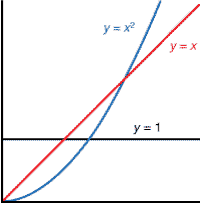
y = 1 (when there was constant acceleration)
y = x (velocity when there is constant acceleration)
y = ½ x2 (displacement when there is constant acceleration)
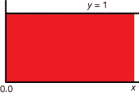
Can you guess what function would give the area shown in red?
Would it be y = 1, y = x, or y = ½ x2?
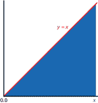
Can you guess what function would give the area shown in blue?
Would it be y = 1, y = x, or y = ½ x2?
You likely found it easy to find the red area and the blue area. You’ve known how to find the area of rectangles and triangles for years. (The red area is y = x; the blue area is y = ½ x2.)
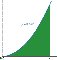
Here is a harder question. What is the area shown in green?
There are no rectangles or triangles to use. So what can you do?
Since someone must have figured this out before, a good first step would be to do some rapid research. You could search the Internet for “area under x squared” and see what you find.
You might also consider the sequence y = 1, y = ½ x2, . . . and try to ascertain the next term. Both of these methods would likely lead you to ![]() .
.

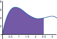
If you are looking for a definite area, such as the ones shown to the left, there are some statistical computer methods that can help.
Quite often you don’t need an exact answer; you just need a close approximation. One numerical way of finding an approximate area is using Monte Carlo Integration. It’s a lot like throwing darts randomly at a board. You count the ones that hit the area you’re interested in. The ratio of the hits to the total lets you find the area.
The Monte Carlo Area applet lets you try this out. Watch out if you have a slower computer—it can take a long time to plot 1 000 000 points. The number of points to try is up to you, but 1000 should work fairly well for everyone.
If you are interested in how the applet works, you can check out the source code here. Finding the area is done in the function gwasplot.
 Module 1: Lesson 4 Assignment
Remember to submit the Module 1: Lesson 4 Assignment to your teacher.
Add to the KWL chart you worked on in Lessons 1 to 3. Continue to store your chart in your Physics 20 course folder.