Module 1—Motion
Part 3: Comparing Observed Motions with Position-Time Graphs
It can be difficult to visualize the motion of an object based on nothing more than a position-time graph. It is also difficult to imagine the graph that represents a motion that you are watching.
You will use a simulation to visualize and compare the actual motion of an object with its representative position-time graph.
You can learn more about the simulation and how to use it by reading the Show Me found at the top of the simulation screen. Open the 1D Uniform Motion Builder Graphing (pos, vel, acc) simulation. If you cannot see the Play and Pause buttons on the bottom of the page, you may need to adjust the window. Click on the coloured title bar at the top, and drag the window to the upper right-hand corner of your screen. Then expand the window down by holding your cursor on the bottom border, clicking on the double-headed arrow that appears and dragging it down till you clearly see the bottom buttons. You can adjust the side margins in a similar way to remove the unused black areas. It will be convenient to have this window tight to the right side of your screen. After these adjustments, continue with Try This.
 Try This
TR 5. Using the simulation, generate a position-time graph for an object that moves at +5.0 m/s for 5.0 s and then at +10.0 m/s for another 5.0 s.
Step 1: On the simulation, click “Reset” (![]() ) and then “Add” (
) and then “Add” (![]() ) to add an object.
) to add an object.
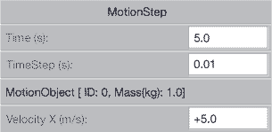
Step 2: In the “MotionStep EditorDialog” window, enter a time of 5.0 s and a velocity of +5.0 m/s. Click OK.

Step 3: Repeat steps 1 and 2, entering a time of 5.0 s and a velocity of +10.0 m/s. Click OK.
Step 4: Click “Play” (![]() ) and watch the moving object (
) and watch the moving object (![]() ) travel at two different velocities.
) travel at two different velocities.
Step 5: To view the position-time graph, do the following:
- Click “Graph.”
![]()
- Set “Horiz. Axis” to “Time” by clicking on the down arrow on the right of the horizontal axis box. Then move the slider on the right up to see “Time” and click on it.
- Set “Vert. Axis” to displacement (x0).

- Click “Fit Graph to the Screen.” (
 ).
).
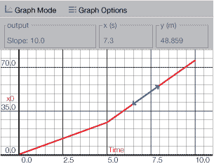
Step 6: To view the slope, expand the graph window by dragging the margin to the right with the double-headed arrow as described earlier until you see the “Slope Mode” button (![]() ). Click the “Slope Mode” button. Click and hold the mouse cursor over the graph line, and the slope value (m/s) will be indicated under Output. You can expand the graph down by dragging the bottom border of the window down and then dragging down the line under the “Zoom Out” button. You can also use the arrows under the “Zoom In” button, but the size adjustment is not as flexible.
). Click the “Slope Mode” button. Click and hold the mouse cursor over the graph line, and the slope value (m/s) will be indicated under Output. You can expand the graph down by dragging the bottom border of the window down and then dragging down the line under the “Zoom Out” button. You can also use the arrows under the “Zoom In” button, but the size adjustment is not as flexible.
Verify that your graph is identical to Figure 2. The slope value is displayed under Output and represents the object’s velocity at the selected time.

Figure 2
 Module 1: Lesson 3 Assignment
Remember to submit the answer to TR 6 to your teacher as part of your Module 1: Lesson 3 Assignment.
TR 6. On the simulation, click “Reset” (![]() ). Clear all motion steps from the simulation by clicking each motion step and clicking “Remove” (
). Clear all motion steps from the simulation by clicking each motion step and clicking “Remove” (![]() ).
).

Enter the following new motion steps on the simulation by clicking “Add” (![]() ):
):
-
5.0 s at +4.0 m/s
-
3.0 s at +14.0 m/s
-
2.0 s at +6.0 m/s
-
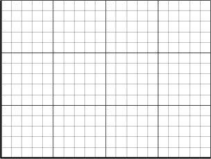
Play the motion, and generate the position-time graph. Draw the graph in the space to the right.
-
Using the “Slope Mode” button, determine and label the velocity for each time interval on your graph.
TR 7. On the simulation, click “Reset” (![]() ). Clear all motion steps from the simulation by clicking each motion
). Clear all motion steps from the simulation by clicking each motion
step and clicking “Remove” (![]() ).
).

Enter the following new motion steps on the simulation by clicking “Add” (![]() ).
).
- 5.0 s at –4.0 m/s
- 3.0 s at +10.0 m/s
- 2.0 s at –2.5 m/s
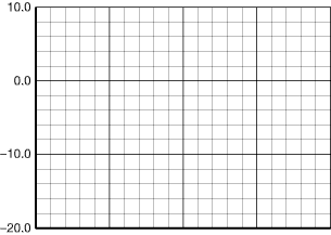
- Play the motion and generate the position-time graph. Draw the graph in the space to the right.
- Using the “Slope Mode” button, determine and label the velocity for each time interval on your graph.