Hemera/Thinkstock
In this module you investigated the following questions:
- How can rational functions be used to solve transportation problems?
- How can function operations be used to simplify transportation problems?
In the first half of this module you explored rational functions, mainly graphically. You determined when both asymptotes and points of discontinuity occurred. You also approximated the solutions to rational equations graphically. The second half of this module focused on function operations. You added, subtracted, multiplied, divided, and composed functions. You also used these operations to solve some problems. In the Module 7 Project: Shipping Wars, you applied an understanding of rational functions and function operations to a transportation business and used these understandings to determine functions that represented various relationships.
Following are some of the key ideas that you learned in each lesson.
Lesson 1 |
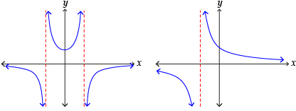
Rational functions can be graphed and transformed in a manner similar to other functions. Many rational functions include asymptotes.
|
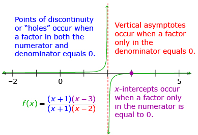
Lesson 2 |
Asymptotes and points of discontinuity are two types of discontinuities that occur at non-permissible values for rational functions.
|
Lesson 3 |
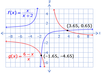
The graphs of rational functions can be used to approximate the solutions to rational equations.
|
Lesson 4 |
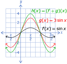
Two functions can be added or subtracted. The notations (f + g)(x) and (f − g)(x) are often used to represent f(x) + g(x) and f(x) − g(x).
Source: Pre-Calculus 12. Whitby, ON: McGraw-Hill Ryerson, 2011. Reproduced with permission.
|
Lesson 5 |
Two functions can be multiplied or divided. The notation (f + g)(x) and |
Lesson 6 |
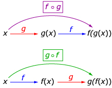
The output from one function can be used as the input for another function by using a composition of functions. The notation (f o g)(x) is often used to represent f(g(x)).
|