Lesson 3 Summary
In this lesson you explored how the graphs of rational functions can be used to solve rational equations. You saw two common methods that you may have used in previous modules or courses for other types of equations. The first method was to graph a function that corresponds to each side of the equation and determine where the functions intersect. The second method was to rewrite the equation so that one side is equal to 0, and then graph the function that corresponds to the other side of the equation and determine the x-intercepts. Both methods typically give approximate solutions.
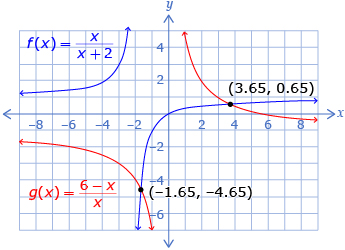
To solve ![]() it is possible to graph
it is possible to graph ![]() and find any intersections.
and find any intersections.
The x-values of these intersections will be the solutions.
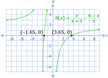
To solve
This is the end of the first half of this module. You explored rational functions. In the second half of this module you will investigate methods of combining separate functions using various function operations.