Explore
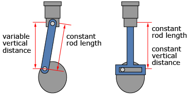
In Try This 1 and Share 1 you explored how two different pistons move over time. The difference in piston motion is due to the first connecting rod “waving” back and forth. This means the vertical distance between the ends of the connecting rod is not always the same. This scenario requires a more complex model than just a sine curve. The second rod does not “wave,” and so the vertical distance between the ends of the rod is constant. The second mechanism can be modelled using the transformations of a sine graph learned so far.
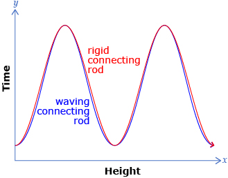
Your sketch of the two graphs should look similar to the following:
The graphs of the two piston heights are a mathematical model of the physical systems. A mathematical model is a representation of a system using mathematical ideas and language. A model is then used to make predictions about the system.
Creating mathematical models that accurately describe phenomena can be a challenging process and is the focus of a branch of mathematics called applied mathematics.
In the piston system, the model was just the sketch of the two graphs. Even though values were not included, it is still possible to determine a lot of information about the system:
- The maximum and minimum values coincide.
- The height of the piston with the waving connecting rod is always less than or equal to the height of the piston with the rigid connecting rod.
- The relative distance between the two heights can be seen.
- The movement of one piston is a close approximation of the movement of the other piston.