In this module you used radical functions to model the relationships between distance, speed, and time for objects as they accelerate. You saw this in objects dropped or thrown, tire skid marks from a vehicle, and the swinging of a pendulum. These relationships were graphed and solved using radical functions.
clock: © asky/2192348/Fotolia; lacross: Hemera/Thinkstock; road: iStockphoto/Thinkstock
You investigated the following question:
- How are radical functions graphed and analyzed to help understand the motion of objects?
You learned how to sketch the graphs of radical functions using your knowledge of transformations from Module 1. The sketches of the graphs of radical functions were made by using the form ![]() and by transforming the function
and by transforming the function ![]() . You also identified the domain and range of the radical functions.
. You also identified the domain and range of the radical functions.
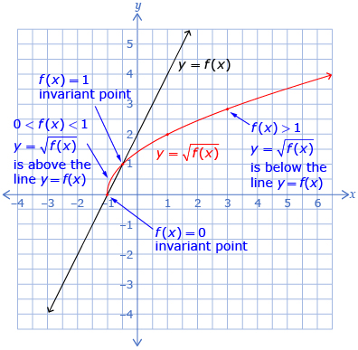
You learned how to sketch the graph of ![]() when given the graph of the function y = f(x). To do this, you used key points and the understanding that the y-coordinates of the function
when given the graph of the function y = f(x). To do this, you used key points and the understanding that the y-coordinates of the function ![]() are the square root of the y-coordinates of the function y = f(x). You also compared the domain and range of each function and explained why the domain and range might be different.
are the square root of the y-coordinates of the function y = f(x). You also compared the domain and range of each function and explained why the domain and range might be different.
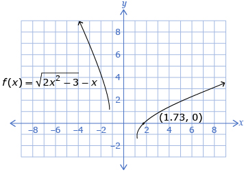
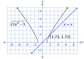
A graphical method was used to solve radical equations. Two methods were studied. One method used a graph of a single function, and the solution was the value of the x-intercept(s). The other method used the graphs of a system of two functions, and the solution was the x-value of the point(s) of intersection.
In Module 2 Project: Pendulums, you applied what you learned in this module to study the relationship between the period and length of a pendulum. You graphed and determined the equation for the function, and you described the transformations of the new function from the base function. You used this equation to determine graphically the period of a pendulum with a given length. You used a graph of a square root of a given function to determine the velocity of a pendulum.
Following are some of the key ideas that you learned in each lesson.
| Lesson 1 | Sketch the graph of
|
| Lesson 2 | Sketch the graph of
|
| Lesson 3 | To solve radical equations graphically, you can use one of two methods to determine the solution.
|