Lesson 2 Summary
In this lesson you looked at the graph of ![]() when given the graph of y = f(x). You can use the values from the function f(x) to predict the values of the function
when given the graph of y = f(x). You can use the values from the function f(x) to predict the values of the function ![]() The y-values of the points of
The y-values of the points of ![]() are the square roots of the y-values of the points on the original function y = f(x).
are the square roots of the y-values of the points on the original function y = f(x).
In terms of mapping: ![]() so
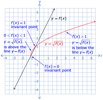
so ![]() The invariant points occur when f(x) = 0 and f(x) = 1 because the square root of 0 is 0 and the square root of 1 is 1. The domain of
The invariant points occur when f(x) = 0 and f(x) = 1 because the square root of 0 is 0 and the square root of 1 is 1. The domain of ![]() are the x-values of f(x) for which f(x) is greater than or equal to zero. The range of
are the x-values of f(x) for which f(x) is greater than or equal to zero. The range of ![]() are the y-values in the range of f(x) for which f(x) is defined.
are the y-values in the range of f(x) for which f(x) is defined.
| f(x) | f(x) < 0 | f(x) = 0 | 0 < f(x) < 1 | f(x) = 1 | f(x) > 1 |
Note: Take the square root of the y-values of y = f(x), and the range must be positive. |
Some of the key lesson points are highlighted on the following graph.
In Lesson 3 you will study how the graphs of radical functions can help solve radical equations.