Explore
In Try This 1 you compared the graphs of y = x + 4 and ![]() You may have noticed that the mapping
You may have noticed that the mapping ![]() shows the correspondence between points on the first graph and those points on the second graph.
shows the correspondence between points on the first graph and those points on the second graph.
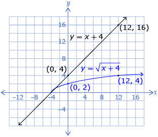
What other patterns do you see when you compare the original function y = x + 4 and the square root of the original function ![]()
In Try This 2 you will compare a given function to the square root of the given function.
Try This 2
Use Visualizing Square Root to compare a function f(x) and the square root of that function ![]()

Comparison 1 has been done for you as an example.
Comparison 1: Compare the functions f(x) = −x + 1 and ![]()
Step 1: Select the linear function in Visualizing Square Root.
Step 2: Use the sliders to set a to −1 and b to 1.
Step 3: Select the "Show Square Root" box and compare the two graphs. Record your observations in a table.
Solution
| f(x) = –x + 1 | ||
| Domain | {x|x ∈ R} | {x|x ≤ 1, x ∈ R} |
| Range | {y|y ∈ R} | {y|y ≥ 0, y ∈ R} |
| Invariant Point(s) |
(1, 0) and (0, 1) | |
| Sketch/Image of Both Functions | 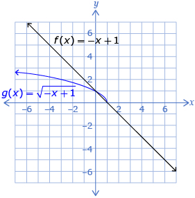 |
|
Comparison 2: Compare the functions f(x) = 0.5x − 1 and ![]()
Step 1: Change a to 0.5 and b to −1.
Step 2: Record your observations in a table similar to the following one.
| f(x) = 0.5x − 1 | ||
| Domain | ||
| Range | ||
| Invariant Point(s) | ||
| Sketch/Image of Both Functions | ||
Comparison 3: Compare the functions f(x) = x2 − 1 and ![]()
Step 1: Change the function to quadratic.
Step 2: Change a to 1, h to 0, and k to −1.
Step 3: Record your observations in a table similar to the following one.
| f(x) = x2 − 1 | ||
| Domain | ||
| Range | ||
| Invariant Point(s) | ||
| Sketch/Image of Both Functions | ||
Comparison 4: Compare the functions f(x) = 3x2 + 4 and ![]()
Step 1: Change a to 3, h to 0, and k to 4.
Step 2: Record your observations in a similar table.
| f(x) = 3x2 + 4 | ||
| Domain | ||
| Range | ||
| Invariant Point(s) | ||
| Sketch/Image of Both Functions | ||
- Look at the location of the invariant points. Is there a pattern? Why are the invariant points located where they are?
- How do the domains compare? Why are there differences?
- How do the ranges compare? Explain the differences.
- Refer to the sketches of each comparison. What happens to the value of
 as the value of f(x) changes? Use the following table to summarize the common patterns you observed for all four comparisons.
Value of f(x)
(original graph)When the y values are less than 0
(f(x) < 0)When the y value is 0
(f(x) = 0)When the y values are between 0 and 1
(0 < f(x) < 1)When the y value is 1
(f(x) = 1)When the y values are greater than 1
(f(x) > 1)Value of 
![]() Save your responses in your course folder.
Save your responses in your course folder.
Share 2
With a partner or group, discuss the following questions based on your graphs created in Try This 2:
Based on the patterns you identified in Try This 2, create a method you could use to graph the square root of any function.
![]() If required, save a record of your discussion in your course folder.
If required, save a record of your discussion in your course folder.